PCA Analysis using tidymodels

Author

Lindsay N. Hayes

Published

July 14, 2025

About the activity

Access the Quarto document here.
Download the raw file.
Open it in RStudio.

We will work our way through this quarto document together during class. The activity will cover Principal Component Analysis (PCA) using tidymodels.

Load the Packages

library(tidyverse)
library(tidymodels)
library(palmerpenguins)

`glimpse` at the data

glimpse(penguins)

Rows: 344
Columns: 8
$ species           <fct> Adelie, Adelie, Adelie, Adelie, Adelie, Adelie, Adel…
$ island            <fct> Torgersen, Torgersen, Torgersen, Torgersen, Torgerse…
$ bill_length_mm    <dbl> 39.1, 39.5, 40.3, NA, 36.7, 39.3, 38.9, 39.2, 34.1, …
$ bill_depth_mm     <dbl> 18.7, 17.4, 18.0, NA, 19.3, 20.6, 17.8, 19.6, 18.1, …
$ flipper_length_mm <int> 181, 186, 195, NA, 193, 190, 181, 195, 193, 190, 186…
$ body_mass_g       <int> 3750, 3800, 3250, NA, 3450, 3650, 3625, 4675, 3475, …
$ sex               <fct> male, female, female, NA, female, male, female, male…
$ year              <int> 2007, 2007, 2007, 2007, 2007, 2007, 2007, 2007, 2007…

Prep the Data and Perform the PCA

# set a seed. Not really necessary for PCA because it is a reproducible analysis and doesn't use random data to model the data. But it is good practice. You can use any number your heart desires. 

set.seed(956)

# don't need to split data for the PCA because its an exploratory data analysis and we want to use all the data. 


# Build a Recipe: this is an instruction manual does not perform any actual analysis, yet. 

penguin_recipe <-
  
  # we want to use all the data to build the analysis so we us ~  and . to include all data numeric variables
  recipe( ~ ., data = penguins) %>% 
  
  # we want to maintain the categorical data so we give it a new rol of id to identify the data
  update_role(species, island, sex, new_role = "id") %>% 
  
  # we want to omit rows with missing data because it can't be properly used by the PCA
  step_naomit(all_predictors()) %>% 
  
  # to make sure all the data is normally distributed and centered we want to normalize the data before running PCA
  step_normalize(all_predictors()) %>%
  
  # finally we want to actually run a PCA analysis on all the data or predictors
  step_pca(all_predictors(), id = "pca")

penguin_recipe

── Recipe ──────────────────────────────────────────────────────────────────────

── Inputs

Number of variables by role

predictor: 5
id:        3

── Operations

• Removing rows with NA values in: all_predictors()

• Centering and scaling for: all_predictors()

• PCA extraction with: all_predictors()

# Prep Data: pull in the variables from the penguins data and runs PCA

penguin_prep <- prep(penguin_recipe, penguins)

penguin_prep

── Recipe ──────────────────────────────────────────────────────────────────────

── Inputs

Number of variables by role

predictor: 5
id:        3

── Training information

Training data contained 344 data points and 11 incomplete rows.

── Operations

• Removing rows with NA values in: bill_length_mm, ... | Trained

• Centering and scaling for: bill_length_mm bill_depth_mm, ... | Trained

• PCA extraction with: bill_length_mm bill_depth_mm, ... | Trained

penguin_prep %>% tidy(id = "pca", type = "coef")

# A tibble: 25 × 4
   terms               value component id   
   <chr>               <dbl> <chr>     <chr>
 1 bill_length_mm     0.452  PC1       pca  
 2 bill_depth_mm     -0.398  PC1       pca  
 3 flipper_length_mm  0.576  PC1       pca  
 4 body_mass_g        0.544  PC1       pca  
 5 year               0.0957 PC1       pca  
 6 bill_length_mm    -0.0935 PC2       pca  
 7 bill_depth_mm      0.0164 PC2       pca  
 8 flipper_length_mm  0.0256 PC2       pca  
 9 body_mass_g       -0.111  PC2       pca  
10 year               0.989  PC2       pca  
# ℹ 15 more rows

penguin_prep %>% tidy(id = "pca", type = "variance")

# A tibble: 20 × 4
   terms                          value component id   
   <chr>                          <dbl>     <int> <chr>
 1 variance                      2.77           1 pca  
 2 variance                      0.993          2 pca  
 3 variance                      0.772          3 pca  
 4 variance                      0.365          4 pca  
 5 variance                      0.0993         5 pca  
 6 cumulative variance           2.77           1 pca  
 7 cumulative variance           3.76           2 pca  
 8 cumulative variance           4.54           3 pca  
 9 cumulative variance           4.90           4 pca  
10 cumulative variance           5.00           5 pca  
11 percent variance             55.4            1 pca  
12 percent variance             19.9            2 pca  
13 percent variance             15.4            3 pca  
14 percent variance              7.30           4 pca  
15 percent variance              1.99           5 pca  
16 cumulative percent variance  55.4            1 pca  
17 cumulative percent variance  75.3            2 pca  
18 cumulative percent variance  90.7            3 pca  
19 cumulative percent variance  98.0            4 pca  
20 cumulative percent variance 100              5 pca

# Bake Data: Extract the data from the PCA

penguin_bake <- bake(penguin_prep, new_data = NULL)

penguin_bake

# A tibble: 342 × 8
   species island    sex       PC1    PC2     PC3     PC4     PC5
   <fct>   <fct>     <fct>   <dbl>  <dbl>   <dbl>   <dbl>   <dbl>
 1 Adelie  Torgersen male   -1.95  -1.12   0.0126  0.241   0.405 
 2 Adelie  Torgersen female -1.42  -1.14   0.489   0.0379  0.280 
 3 Adelie  Torgersen female -1.48  -1.06   0.209  -0.192  -0.643 
 4 Adelie  Torgersen female -1.99  -1.01   0.0549  0.624  -0.591 
 5 Adelie  Torgersen male   -2.02  -1.08  -0.772   0.692  -0.321 
 6 Adelie  Torgersen female -1.87  -1.11   0.411  -0.0192  0.385 
 7 Adelie  Torgersen male   -0.927 -1.22  -0.458   1.34    0.213 
 8 Adelie  Torgersen <NA>   -1.94  -0.983  0.821   0.695  -0.543 
 9 Adelie  Torgersen <NA>   -1.31  -1.21  -0.962   0.737   0.212 
10 Adelie  Torgersen <NA>   -1.84  -1.04   0.844  -0.198  -0.0969
# ℹ 332 more rows

Evaluate the PCA

# tidy type can be: "coef", "variance", 

# Plot the percent of variance explained by each principal component
penguin_prep %>% 
  tidy(id = "pca", type = "variance") |> 
  dplyr::filter(terms == "percent variance") |> 
  ggplot(aes(x = component, y = value)) + 
  geom_col(fill = "#b6dfe2") + 
  xlim(c(0, 5)) + 
  ylab("% of total variance") +
   geom_text(aes(label=round(value,1)), vjust = 1.5)

Warning: Removed 1 row containing missing values or values outside the scale range
(`geom_col()`).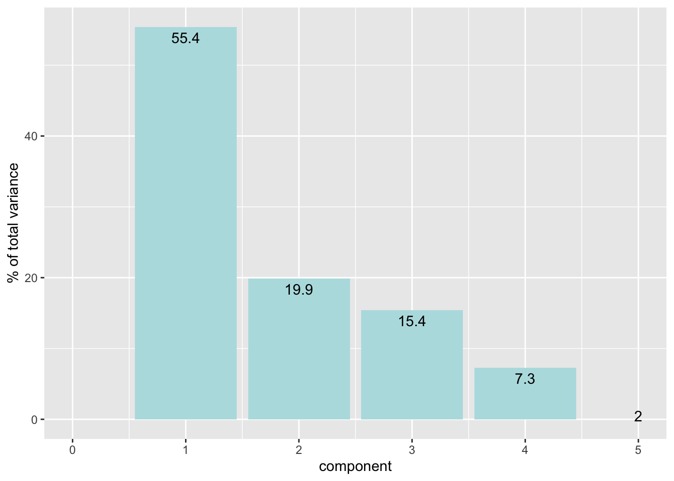

# Plot which predictors/variables are explained in each principal component
penguin_prep |>
  tidy(id = "pca", type = "coef") |> 
  ggplot(aes(abs(value), terms, fill = value > 0)) +
  geom_col() +
  facet_wrap(~component, scales = "free_y") +
  scale_fill_manual(values = c("#b6dfe2", "#0A537D")) +
  labs(
    x = "Absolute value of contribution",
    y = NULL, fill = "Pos Affil")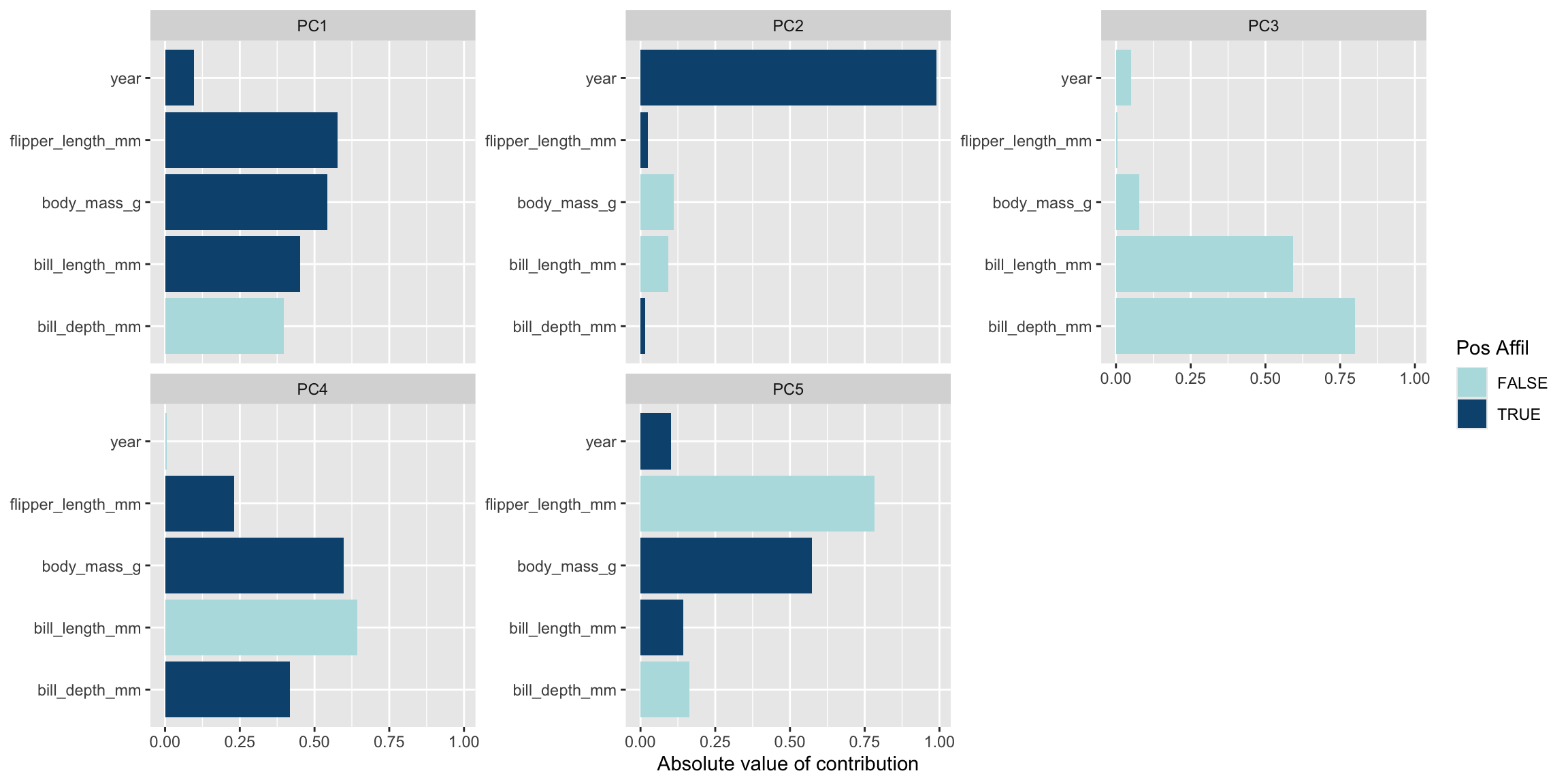

# Plot the PCA
pca_plot <- penguin_bake |> 
  ggplot(aes(PC1, PC2)) +
  geom_point(aes(color = species, shape = species), 
             alpha = 0.8, 
             size = 2) +
  scale_colour_manual(values = c("darkorange","purple","cyan4")) +
  theme_bw()

pca_plot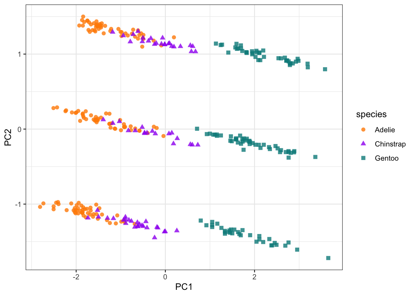

# Add the vectors for how the variables are explained by each PC

pca_wider <- penguin_prep |> 
              tidy(id = "pca", type = "coef") |>
              pivot_wider(names_from = component, id_cols = terms)

arrow_style <- arrow(length = unit(.05, "inches"), type = "closed")

pca_plot +
  geom_segment(data = pca_wider,
               aes(xend = PC1, yend = PC2), 
               x = 0, 
               y = 0, 
               arrow = arrow_style) + 
  geom_text(data = pca_wider,
            aes(x = PC1, y = PC2, label = terms), 
            hjust = 0, 
            vjust = 1,
            size = 5, 
            color = '#0A537D')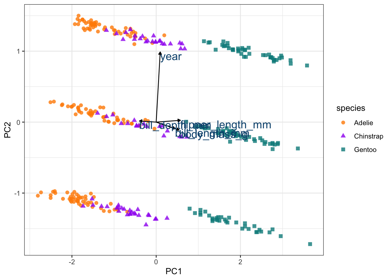

We can see that year is having a large impact of PC2 and obscuring the effect of the other metrics. So we can exclude PC2 and plot PC1 and PC3 instead.

pca_plot <- penguin_bake |> 
  ggplot(aes(PC1, PC3)) +
  geom_point(aes(color = species, shape = species), 
             alpha = 0.8, 
             size = 2) +
  scale_colour_manual(values = c("darkorange","purple","cyan4")) +
  theme_bw()

pca_plot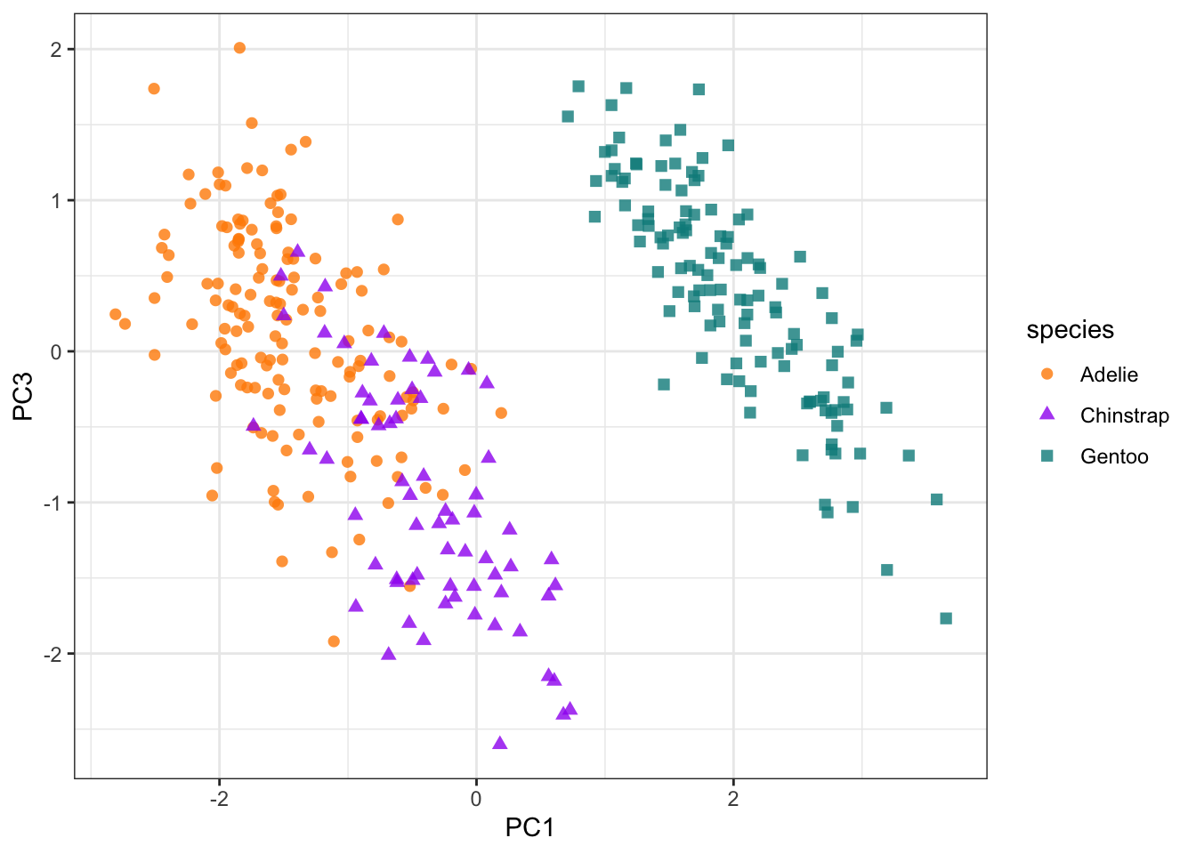

arrow_style <- arrow(length = unit(.05, "inches"), type = "closed")

pca_plot +
  geom_segment(data = pca_wider,
               aes(xend = PC1, yend = PC3), 
               x = 0, 
               y = 0, 
               arrow = arrow_style) + 
  geom_text(data = pca_wider,
            aes(x = PC1, y = PC3, label = terms), 
            hjust = 0, 
            vjust = 1,
            size = 5, 
            color = '#0A537D')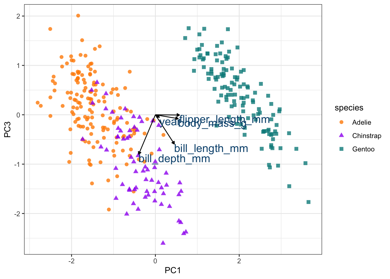

sessionInfo()

R version 4.4.1 (2024-06-14)
Platform: aarch64-apple-darwin20
Running under: macOS Sonoma 14.5

Matrix products: default
BLAS:   /Library/Frameworks/R.framework/Versions/4.4-arm64/Resources/lib/libRblas.0.dylib 
LAPACK: /Library/Frameworks/R.framework/Versions/4.4-arm64/Resources/lib/libRlapack.dylib;  LAPACK version 3.12.0

locale:
[1] en_US.UTF-8/en_US.UTF-8/en_US.UTF-8/C/en_US.UTF-8/en_US.UTF-8

time zone: America/Chicago
tzcode source: internal

attached base packages:
[1] stats     graphics  grDevices utils     datasets  methods   base     

other attached packages:
 [1] palmerpenguins_0.1.1 yardstick_1.3.2      workflowsets_1.1.1  
 [4] workflows_1.2.0      tune_1.3.0           rsample_1.3.0       
 [7] recipes_1.3.1        parsnip_1.3.2        modeldata_1.4.0     
[10] infer_1.0.8          dials_1.4.0          scales_1.3.0        
[13] broom_1.0.7          tidymodels_1.3.0     lubridate_1.9.4     
[16] forcats_1.0.0        stringr_1.5.1        dplyr_1.1.4         
[19] purrr_1.0.4          readr_2.1.5          tidyr_1.3.1         
[22] tibble_3.2.1         ggplot2_3.5.2        tidyverse_2.0.0     

loaded via a namespace (and not attached):
 [1] tidyselect_1.2.1    timeDate_4041.110   farver_2.1.2       
 [4] fastmap_1.2.0       digest_0.6.37       rpart_4.1.24       
 [7] timechange_0.3.0    lifecycle_1.0.4     survival_3.8-3     
[10] magrittr_2.0.3      compiler_4.4.1      rlang_1.1.5        
[13] tools_4.4.1         utf8_1.2.4          yaml_2.3.10        
[16] data.table_1.17.0   knitr_1.50          labeling_0.4.3     
[19] htmlwidgets_1.6.4   DiceDesign_1.10     withr_3.0.2        
[22] nnet_7.3-20         grid_4.4.1          colorspace_2.1-1   
[25] future_1.49.0       globals_0.18.0      iterators_1.0.14   
[28] MASS_7.3-64         cli_3.6.4           rmarkdown_2.29     
[31] generics_0.1.3      rstudioapi_0.17.1   future.apply_1.11.3
[34] tzdb_0.4.0          splines_4.4.1       parallel_4.4.1     
[37] vctrs_0.6.5         hardhat_1.4.1       Matrix_1.7-2       
[40] jsonlite_1.9.1      hms_1.1.3           listenv_0.9.1      
[43] foreach_1.5.2       gower_1.0.2         glue_1.8.0         
[46] parallelly_1.45.0   codetools_0.2-20    stringi_1.8.4      
[49] gtable_0.3.6        munsell_0.5.1       GPfit_1.0-9        
[52] pillar_1.10.1       furrr_0.3.1         htmltools_0.5.8.1  
[55] ipred_0.9-15        lava_1.8.1          R6_2.6.1           
[58] lhs_1.2.0           evaluate_1.0.3      lattice_0.22-6     
[61] backports_1.5.0     class_7.3-23        Rcpp_1.0.14        
[64] prodlim_2024.06.25  xfun_0.51           pkgconfig_2.0.3

About the activity

Load the Packages

glimpse at the data

Prep the Data and Perform the PCA

Evaluate the PCA

We can see that year is having a large impact of PC2 and obscuring the effect of the other metrics. So we can exclude PC2 and plot PC1 and PC3 instead.

`glimpse` at the data